A fitness function is a particular type of objective function that is used to summarise, as a single figure of merit, how close a given design solution is to achieving the set aims.
In particular, in the fields of genetic programming and genetic algorithms, each design solution is commonly represented as a string of numbers (referred to as a chromosome). After each round of testing, or simulation, the idea is to delete the 'n' worst design solutions, and to breed 'n' new ones from the best design solutions. Each design solution, therefore, needs to be awarded a figure of merit, to indicate how close it came to meeting the overall specification, and this is generated by applying the fitness function to the test, or simulation, results obtained from that solution.
The reason that genetic algorithms cannot be considered to be a lazy way of performing design work is precisely because of the effort involved in designing a workable fitness function. Even though it is no longer the human designer, but the computer, that comes up with the final design, it is the human designer who has to design the fitness function. If this is designed badly, the algorithm will either converge on an inappropriate solution, or will have difficulty converging at all.
Moreover, the fitness function must not only correlate closely with the designer's goal, it must also be computed quickly. Speed of execution is very important, as a typical genetic algorithm must be iterated many times in order to produce a usable result for a non-trivial problem.
Fitness approximation may be appropriate, especially in the following cases:
- Fitness computation time of a single solution is extremely high
- Precise model for fitness computation is missing
- The fitness function is uncertain or noisy.
Two main classes of fitness functions exist: one where the fitness function does not change, as in optimizing a fixed function or testing with a fixed set of test cases; and one where the fitness function is mutable, as in niche differentiation or co-evolving the set of test cases.
Another way of looking at fitness functions is in terms of a fitness landscape, which shows the fitness for each possible chromosome.
Definition of the fitness function is not straightforward in many cases and often is performed iteratively if the fittest solutions produced by GA are not what is desired. In some cases, it is very hard or impossible to come up even with a guess of what fitness function definition might be. Interactive genetic algorithms address this difficulty by outsourcing In applied mathematics, test functions, known as artificial landscapes, are useful to evaluate characteristics of optimization algorithms, such as:
- Convergence rate.
- Precision.
- Robustness.
- General performance.
Here some test functions are presented with the aim of giving an idea about the different situations that optimization algorithms have to face when coping with these kinds of problems. In the first part, some objective functions for single-objective optimization cases are presented. In the second part, test functions with their respective Pareto fronts for multi-objective optimization problems (MOP) are given.
The artificial landscapes presented herein for single-objective optimization problems are taken from Bäck,[1] Haupt et al.[2] and from Rody Oldenhuis software.[3] Given the number of problems (55 in total), just a few are presented here. The complete list of test functions is found on the Mathworks website.[4]
The test functions used to evaluate the algorithms for MOP were taken from Deb,[5] Binh et al.[6] and Binh.[7] You can download the software developed by Deb,[8] which implements the NSGA-II procedure with GAs, or the program posted on Internet,[9] which implements the NSGA-II procedure with ES.
Just a general form of the equation, a plot of the objective function, boundaries of the object variables and the coordinates of global minima are given herein.
Contents
[hide]Test functions for single-objective optimization[edit]
| Name | Plot | Formula | Global minimum | Search domain |
|---|---|---|---|---|
| Rastrigin function |  | |||
| Ackley's function | 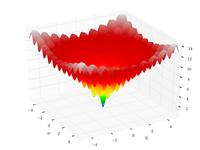 | |||
| Sphere function | 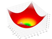 | , | ||
| Rosenbrock function | 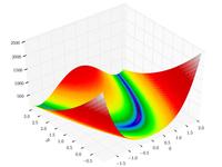 | , | ||
| Beale's function |  | |||
| Goldstein–Price function | 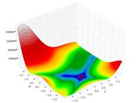 | |||
| Booth's function | 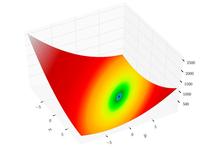 | |||
| Bukin function N.6 | 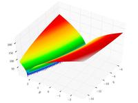 | , | ||
| Matyas function | 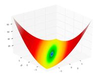 | |||
| Lévi function N.13 | 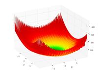 | |||
| Three-hump camel function | 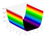 | |||
| Easom function | 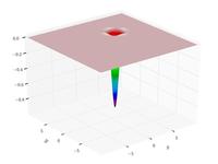 | |||
| Cross-in-tray function | 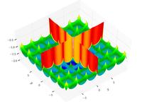 | |||
| Eggholder function | 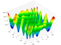 | |||
| Hölder table function | 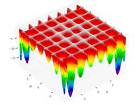 | |||
| McCormick function | 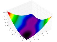 | , | ||
| Schaffer function N. 2 | 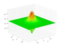 | |||
| Schaffer function N. 4 | 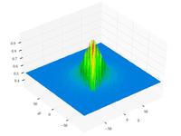 | |||
| Styblinski–Tang function | 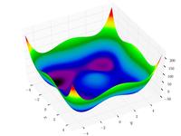 | , .. |
![f(\mathbf {x} )=An+\sum _{i=1}^{n}\left[x_{i}^{2}-A\cos(2\pi x_{i})\right]](https://wikimedia.org/api/rest_v1/media/math/render/svg/1aa1c38ee739ca9cf4582867d74d469df4676cbc)


![{\displaystyle f(x,y)=-20\exp \left[-0.2{\sqrt {0.5\left(x^{2}+y^{2}\right)}}\right]}](https://wikimedia.org/api/rest_v1/media/math/render/svg/7f00d1325d65d088f8ae6a96137e62021107921d)
![{\displaystyle -\exp \left[0.5\left(\cos 2\pi x+\cos 2\pi y\right)\right]+e+20}](https://wikimedia.org/api/rest_v1/media/math/render/svg/565ef43958a50fb0ef473bdd46e30bfc725604a7)


![f({\boldsymbol {x}})=\sum _{i=1}^{n-1}\left[100\left(x_{i+1}-x_{i}^{2}\right)^{2}+\left(x_{i}-1\right)^{2}\right]](https://wikimedia.org/api/rest_v1/media/math/render/svg/5ac655db50e19ee2f79a97196565e8773cd7d659)


![{\displaystyle f(x,y)=\left[1+\left(x+y+1\right)^{2}\left(19-14x+3x^{2}-14y+6xy+3y^{2}\right)\right]}](https://wikimedia.org/api/rest_v1/media/math/render/svg/2d020ed324ff07759faf17591157771b0e2cdf07)
![{\displaystyle \left[30+\left(2x-3y\right)^{2}\left(18-32x+12x^{2}+48y-36xy+27y^{2}\right)\right]}](https://wikimedia.org/api/rest_v1/media/math/render/svg/32e562da4f3219f9d66e059441c59e1d299e8557)


![{\displaystyle f(x,y)=-0.0001\left[\left|\sin x\sin y\exp \left(\left|100-{\frac {\sqrt {x^{2}+y^{2}}}{\pi }}\right|\right)\right|+1\right]^{0.1}}](https://wikimedia.org/api/rest_v1/media/math/render/svg/d591ae9bcf2feae162cd00398d78bb6870c82946)


![{\displaystyle f(x,y)=0.5+{\frac {\sin ^{2}\left(x^{2}-y^{2}\right)-0.5}{\left[1+0.001\left(x^{2}+y^{2}\right)\right]^{2}}}}](https://wikimedia.org/api/rest_v1/media/math/render/svg/995008c6f10a14b44dac568cc544efb7d5ddd631)
![{\displaystyle f(x,y)=0.5+{\frac {\cos ^{2}\left[\sin \left(\left|x^{2}-y^{2}\right|\right)\right]-0.5}{\left[1+0.001\left(x^{2}+y^{2}\right)\right]^{2}}}}](https://wikimedia.org/api/rest_v1/media/math/render/svg/2458c352c0c0524648d8ef713bcea4e80df32fd8)


Test functions for constrained optimization[edit]
| Name | Plot | Formula | Global minimum | Search domain |
|---|---|---|---|---|
| Rosenbrock function constrained with a cubic and a line[10] |  | ,
subjected to:
| , | |
| Rosenbrock function constrained to a disk[11] |  | ,
subjected to:
| , | |
| Mishra's Bird function - constrained[12] |  | ,
subjected to:
| , | |
| Townsend function[13] |  | ,
subjected to: where: t = Atan2(y/x)
| , | |
| Simionescu function[14] |  | ,
subjected to:
|


![{\displaystyle f(x,y)=-[\cos((x-0.1)y)]^{2}-x\sin(3x+y)}](https://wikimedia.org/api/rest_v1/media/math/render/svg/8dac25f97d0b720512d72c313000d5fb5c7d033a)
![{\displaystyle x^{2}+y^{2}<[2\cos t-0.5\cos 2t-0.25\cos 3t-0.125\cos 4t]^{2}+[2\sin t]^{2}}](https://wikimedia.org/api/rest_v1/media/math/render/svg/c2d7b247d7ab7e8348454340b3e8d7cc6aa17e0c)


![{\displaystyle x^{2}+y^{2}\leq \left[r_{T}+r_{S}\cos \left(n\arctan {\frac {x}{y}}\right)\right]^{2}}](https://wikimedia.org/api/rest_v1/media/math/render/svg/1fc42adcc2095ed0c0214a74799db7ee2fac9923)


Test functions for multi-objective optimization[edit]
| Name | Plot | Functions | Constraints | Search domain |
|---|---|---|---|---|
| Binh and Korn function: | 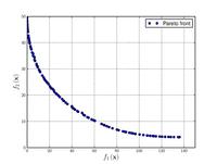 | , | ||
| Chakong and Haimes function: |  | |||
| Fonseca and Fleming function:[15] | 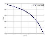 | , | ||
| Test function 4:[7] | ![Test function 4.[7]](https://upload.wikimedia.org/wikipedia/commons/thumb/3/3c/Test_function_4_-_Binh.pdf/page1-200px-Test_function_4_-_Binh.pdf.jpg) | |||
| Kursawe function:[16] | 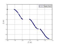 | , . | ||
| Schaffer function N. 1:[17] | 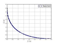 | . Values of from to have been used successfully. Higher values of increase the difficulty of the problem. | ||
| Schaffer function N. 2: |  | . | ||
| Poloni's two objective function: | 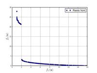 | |||
| Zitzler–Deb–Thiele's function N. 1: |  | , . | ||
| Zitzler–Deb–Thiele's function N. 2: | 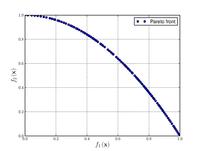 | , . | ||
| Zitzler–Deb–Thiele's function N. 3: | 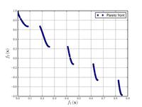 | , . | ||
| Zitzler–Deb–Thiele's function N. 4: | 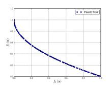 | , , | ||
| Zitzler–Deb–Thiele's function N. 6: |  | , . | ||
| Viennet function: | 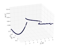 | . | ||
| Osyczka and Kundu function: | 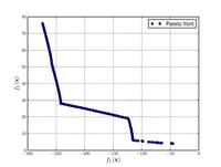 | , , . | ||
| CTP1 function (2 variables):[5] | ![CTP1 function (2 variables).[5]](https://upload.wikimedia.org/wikipedia/commons/thumb/d/d4/CTP1_function_%282_variables%29.pdf/page1-200px-CTP1_function_%282_variables%29.pdf.jpg) | . | ||
| Constr-Ex problem:[5] | ![Constr-Ex problem.[5]](https://upload.wikimedia.org/wikipedia/commons/thumb/6/6f/Constr-Ex_problem.pdf/page1-200px-Constr-Ex_problem.pdf.jpg) |


![{\displaystyle {\text{Minimize}}={\begin{cases}f_{1}\left({\boldsymbol {x}}\right)&=1-\exp \left[-\sum _{i=1}^{n}\left(x_{i}-{\frac {1}{\sqrt {n}}}\right)^{2}\right]\\f_{2}\left({\boldsymbol {x}}\right)&=1-\exp \left[-\sum _{i=1}^{n}\left(x_{i}+{\frac {1}{\sqrt {n}}}\right)^{2}\right]\\\end{cases}}}](https://wikimedia.org/api/rest_v1/media/math/render/svg/52a5ad8aa87005e092dcf8e258abf0842fc7d996)


![{\text{Minimize}}={\begin{cases}f_{1}\left({\boldsymbol {x}}\right)&=\sum _{i=1}^{2}\left[-10\exp \left(-0.2{\sqrt {x_{i}^{2}+x_{i+1}^{2}}}\right)\right]\\&\\f_{2}\left({\boldsymbol {x}}\right)&=\sum _{i=1}^{3}\left[\left|x_{i}\right|^{0.8}+5\sin \left(x_{i}^{3}\right)\right]\\\end{cases}}](https://wikimedia.org/api/rest_v1/media/math/render/svg/a545df8c08a178973284eae8924aab67ce46077a)


![{\text{Minimize}}={\begin{cases}f_{1}\left(x,y\right)&=\left[1+\left(A_{1}-B_{1}\left(x,y\right)\right)^{2}+\left(A_{2}-B_{2}\left(x,y\right)\right)^{2}\right]\\f_{2}\left(x,y\right)&=\left(x+3\right)^{2}+\left(y+1\right)^{2}\\\end{cases}}](https://wikimedia.org/api/rest_v1/media/math/render/svg/e6b4a1275cbe615b285fbbcdb840a9a488360cc5)


![{\text{Minimize}}={\begin{cases}f_{1}\left({\boldsymbol {x}}\right)&=1-\exp \left(-4x_{1}\right)\sin ^{6}\left(6\pi x_{1}\right)\\f_{2}\left({\boldsymbol {x}}\right)&=g\left({\boldsymbol {x}}\right)h\left(f_{1}\left({\boldsymbol {x}}\right),g\left({\boldsymbol {x}}\right)\right)\\g\left({\boldsymbol {x}}\right)&=1+9\left[{\frac {\sum _{i=2}^{10}x_{i}}{9}}\right]^{0.25}\\h\left(f_{1}\left({\boldsymbol {x}}\right),g\left({\boldsymbol {x}}\right)\right)&=1-\left({\frac {f_{1}\left({\boldsymbol {x}}\right)}{g\left({\boldsymbol {x}}\right)}}\right)^{2}\\\end{cases}}](https://wikimedia.org/api/rest_v1/media/math/render/svg/73a519e6f7ca429b41031cd0873fce161941b009)


No comments:
Post a Comment